Today we will tackle a very important concept related to GGPLOT2’s geometries (geom_): the stat = input of geom_ and the stat_ function.
But, what are we referring to with stat? Stat stands for statistics, and it concerns the statistical transformations behind every geom_ command. In fact, each geom_ command is associated with a basic statistic that associates an y value to each x value.
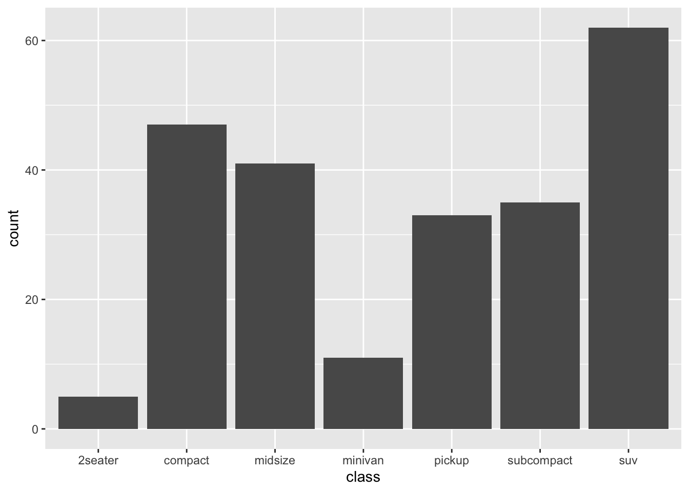
geom_bar (aes (x = class)) in the mpg dataset.

Figure 1: geom_bar example
The function produced a barplot of the frequencies of the various classes, with the y-axis representing the counts (number of occurrences) of each class.
Let’s now analyze the characteristics of stat.
Default statistics
First, let’s analyze the stat = input of the geom_ function.
As mentioned previously, a statistic is associated with each geom_. We are not going to analyze them all, the complete list can be found in the default statistics table at the bottom of the page.
Let’s start from the example 1: the statistic associated with geom_bar is stat_count, i.e. the occurrences of each class in the dataset are plotted on the y axis.
In the table, you can see how many geom_ are associated with stat_identity, what does this mean? It means that in these cases it is necessary to supply both x and y in aes() and that the function will plot each y value over the corresponding x value.
Use a different statistic
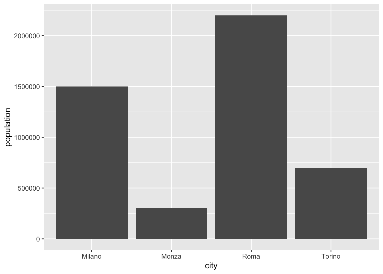
Obviously, the default statistics can be replaced if necessary.geom_bar(aes(x, y), stat = "identity"). The result would be:

Figure 2: Changing stat allowes two vectors to be the inputs of geom_bar
If you were to omit stat =" identity ", you would get an error.
NB: the geom_col function does the same job, without the need of the stat specification, as its default is identity.
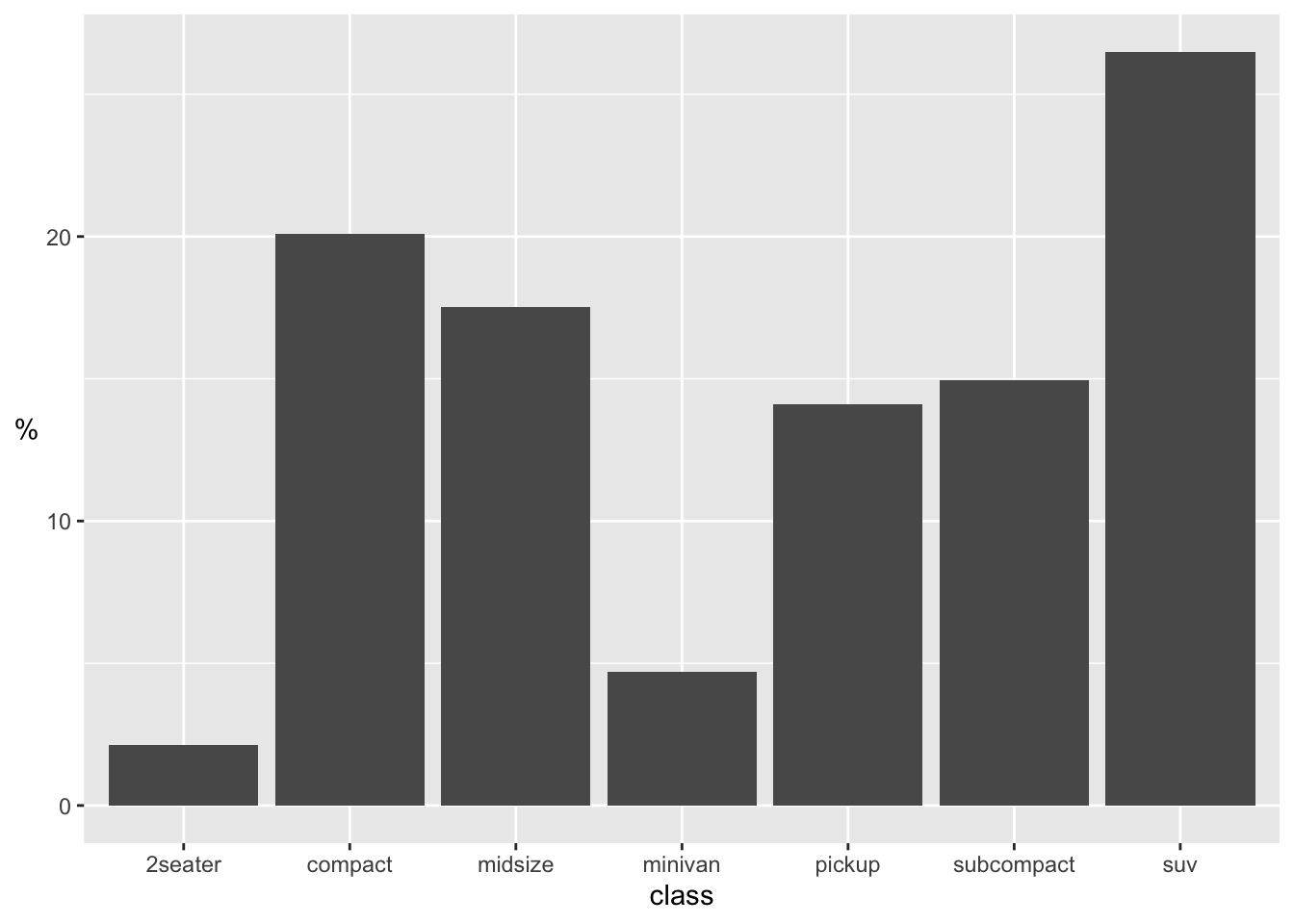
y = after_stat () and make it do any operation inside, with no need to add stat = after.
geom_bar(aes(x = class, y = after_stat(100 * count / sum (count)))):

Figure 3: Using after_stat allow to do mathematical operations
stat_ function
Stat is also a function of ggplot2, with the <stat_function> structure, which can either replace geom_ or add something to the graph.
In fact, as you can see in the complementary table, many geom_ can be replaced by a corresponding stat_ function.
For example, the graph in figure 1 can be obtained also using the command ggplot (mpg) + stat_count (aes (x = class)). However, by convention, we always use geom_ when possible and use the stat_ function only when there are no possible geom_.
In the default geometry table there is the list of possible stat_ functions, with the associated default geometry.
Let’s immediately see an example.
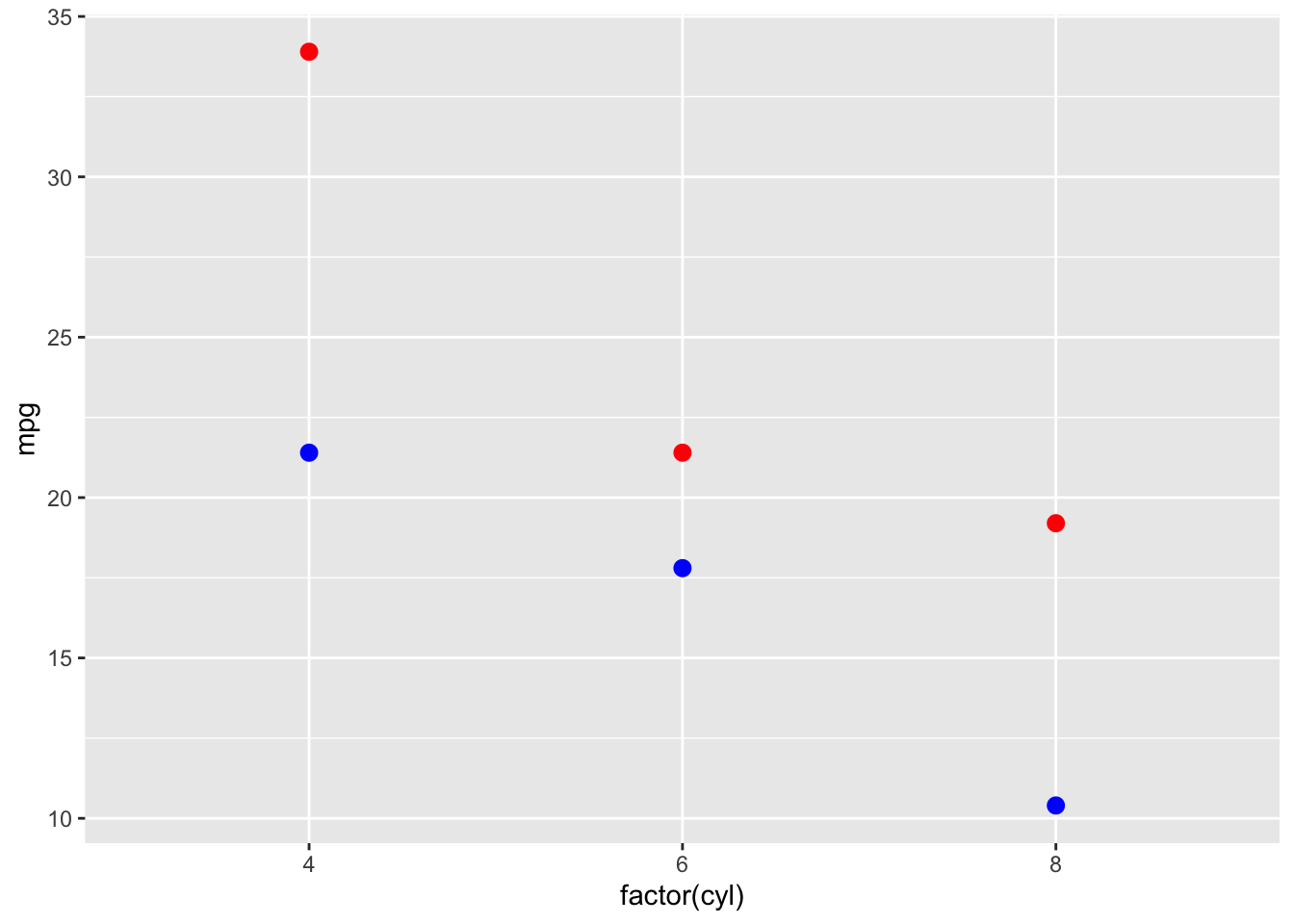
stat_summary. In this case we plot the points corresponding to the minimum and maximum horsepower (hp) values for the three subgroups of cars (mtcars dataset), grouped on the basis of the number of cylinders (cyl).
ggplot(mtcars) +
  stat_summary(aes(x = factor(cyl), y = mpg), fun = min, color = "blue") +
stat_summary(aes(x = factor(cyl), y = mpg), fun = max, color = "red") 
Figure 4: stat_summary example
There are countless uses for the various stat functions, for this I refer to the corresponding documentation. This post was mainly used to illustrate, with some examples, how to exploit the stat component of ggplot2.
Tables
Default statistics
| Geom | Default statistics |
|---|---|
| geom_abline() | stat_identity() |
| geom_area() | stat_identity() |
| geom_bar() | stat_count() |
| geom_bin2d() | stat_bin_2d() |
| geom_blank() | None |
| geom_boxplot() | stat_boxplot() |
| geom_col() | stat_identity() |
| geom_count() | stat_sum() |
| geom_countour_filled() | stat_countour_filled() |
| geom_countour() | stat_countour() |
| geom_crossbar() | stat_identity() |
| geom_curve() | stat_identity() |
| geom_density_2d_filled() | stat_density_2d_filled() |
| geom_density_2d() | stat_density_2d() |
| geom_density() | stat_density() |
| geom_dotplot() | stat_bindot() |
| geom_errorbar() | stat_identity() |
| geom_errorbarh() | stat_identity() |
| geom_freqpoly() | stat_bin() |
| geom_function() | stat_function() |
| geom_hex() | stat_bin_hex() |
| geom_histogram() | stat_bin() |
| geom_hline() | stat_identity() |
| geom_jitter() | stat_identity() |
| geom_label() | stat_identity() |
| geom_line() | stat_identity() |
| geom_linerange() | stat_identity() |
| geom_map() | stat_identity() |
| geom_path() | stat_identity() |
| geom_point() | stat_identity() |
| geom_pointrange() | stat_identity() |
| geom_polygon() | stat_identity() |
| geom_qq_line() | stat_qq_line() |
| geom_qq() | stat_qq() |
| geom_quantile() | stat_quantile() |
| geom_raster() | stat_identity() |
| geom_rect() | stat_identity() |
| geom_ribbon() | stat_identity() |
| geom_rug() | stat_identity() |
| geom_segment() | stat_identity() |
| geom_sf_label() | stat_sf_coordinates() |
| geom_sf_text() | stat_sf_coordinates() |
| geom_sf() | stat_sf() |
| geom_smooth() | stat_smooth() |
| geom_spoke() | stat_identity() |
| geom_step() | stat_identity() |
| geom_text() | stat_identity() |
| geom_tile() | stat_identity() |
| geom_violin() | stat_ydensity() |
| geom_vline() | stat_identity() |
